

The first part of the article in which we established the goals of the experiment, selected factors and their testing levels,, can be found here
What will we measure during DOE?
1. Y, or preferably the main Ys, are numerical metrics describing the effect of the tested factors
We therefore need to measure the yolk quality and ease of peeling. At this point, we assess this only visually, at most commenting on the cooking results. For DOE, we need continuous data. If all we know after the test is whether the egg is good or bad, analysis will be practically impossible. If, for example, our current process only involves visual assessment, we need to find a numerical metric for DOE. There are several ways to do this, but more on that another time.
How will we manage this DOE? We will use Adobe Capture to assess the color. This application will give us a color reading for each egg (after cutting it) in the additive RGB (Reed Green Blue) color model, hence:
Y1 – Yolk Goldenness [Reed/Green]. The R/G ratio is an indicator of the color shift toward warmth. When R is close to G, we have a neutral yellow color. When R<G, the color shifts towards green, meaning a less appetizing yolk. As R>G increases, the color becomes warmer, more golden, and sometimes slightly orange.
Y2 – Green Ring – the G channel value indicates an overcooked egg. The higher the G level, the less appetizing the egg looks.
The next Y will be the comparative scale.
Y3 – Visual Yolk Quality – a scale created after the doe, by arranging the eggs from visually “prettiest” to visually “most overcooked.” Subsequent eggs will be assigned numbers, which will be analyzed as a doe score. The higher the number, the poorer the yolk.
To assess peeling quality, we will use time measurement. Using a stopwatch with a resolution of 0.01 s, we will measure:
Y4 – Peeling Time [s]. Theoretically, the shorter the better, although not necessarily. Therefore, in our doe, we will use a jewelry scale with a resolution of 0.01g to measure the next Y:
Y5 – Shell mass [g]. Increased shell mass means that it did not separate “easily” from the egg white, and some of the egg white may have “gone with the shell.”
2. Other Ys, which may be affected by the tested factors. The idea is simple; it’s easy to improve one Y and ruin the ones that are currently good
Y6 – Weight loss after cooking [%]. Calculated as the ratio of the weight before to after cooking. Theoretically, the weight should not change because the egg only changes state, not volume. In practice, water vapor escapes through pores in the shell, and some of the egg white may dehydrate slightly. For an egg that does not crack (the desired situation), the weight decreases by approximately 0.5 to 2%. If it cracks, the loss will be uch greater. This Y does not directly assess the quality of the yolk or the ease of peeling the egg, but will be an indicator of the quality of the cooking process.
3. Other measurements:
Depending on the situation, we may need to verify the correctness of certain test factors. This is necessary when the test factor has a certain inertia (for example, cooling and heating of a mold, e.g., a casting mold or an injection mold). Additionally, we may want to measure the level of certain interferences during the test, which may be useful during analysis.
Which experimental design should I choose? Full-factorial or fractional design?
To test 6 factors at two levels, we have several options:
- 26 = 64 –a full-factorial design, where 2 is the number of levels, 6 is the number of factors, and 64 is the number of runs
and three options for a fractional design:
- 26-3III=8
- 26-2IV=16
- 26-1VI=32
where 2 is the number of levels, 6 is the number of factors, -1, -2, -3 is the fraction, III, IV, VI is the experiment resolution, and 8, 16, 32 are the number of runs depending on the size of the fraction.
We make our choice based on the number of runs, and if we are considering a fractional experiment, we must also consider the experiment resolution.
In the case of 6 factors, the resources required to conduct a full-factorial experiment are too large. Therefore, we decided on a fractional experiment. We rejected the scenario 26-3III=8, due to resolution III, which is burdened with a high level of entanglement. 26-1VI=32, s still too resource-intensive. Of the three available options, we ultimately chose 26-2IV=16, which is a good compromise between the number of runs and the level of entanglement.
We will write about fractional experiments, entanglement, and resolution another time.
Creating the Experimental Matrix:
After selecting the experimental design, ideally using software (e.g., Minitab, JMP, and many others), create the experimental matrix. In our case, it’s the 26-2IV=16 matrix.
Of course, this can be done manually. For a full-factorial experiment, it’s simple. For fractional experiments, it’s a bit more complicated and subject to a high probability of error—but not impossible. We’ll explain how to do this, but that’s a topic for a completely different OPEX story.
The experimental matrix for our example is presented in the table below.
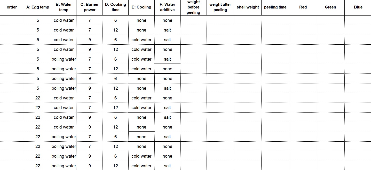
click to enlarge
If you plan to conduct a fractional experiment, save the Confounding Structure. You’ll need it for proper analysis of the experiment.
The Alias Structure for the 26-2IV=16 doe looks as follows:
A + BCE + DEF + ABCDF
B + ACE + CDF + ABDEF
C + ABE + BDF + ACDEF
D + AEF + BCF + ABCDE
E + ABC + ADF + BCDEF
F + ADE + BCD + ABCEF
AB + CE + ACDF + BDEF
AC + BE + ABDF + CDEF
AD + EF + ABCF + BCDE
AE + BC + DF + ABCDEF
AF + DE + ABCD + BCEF
BD + CF + ABEF + ACDE
BF + CD + ABDE + ACEF
ABD + ACF + BEF + CDE
ABF + ACD + BDE + CEF
