

Below you will find the earlier parts of this article:
How to verify the quality of the model?
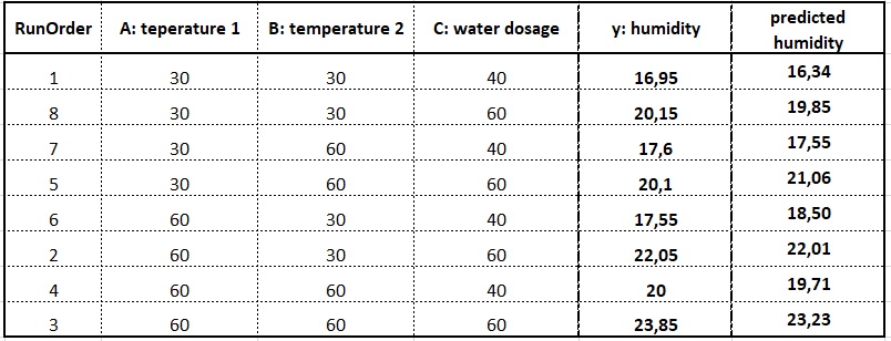
How can we verify how accurately it predicts humidity for different settings of factors A, B, and C, and the AB interaction? It’s best to compare the humidity predicted by the prediction equation with the results we know from doe, i.e., the y we obtained in subsequent runs of the experiment. The table below shows the y obtained from doe and the y predicted by the model for all eight runs of the experiment.
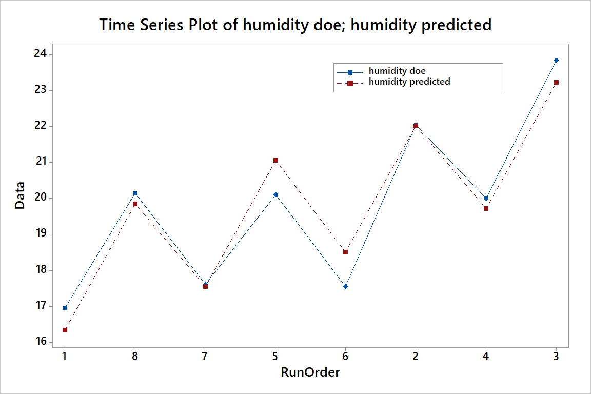
The differences in how the results obtained by the prediction equation differ from those obtained in doe can be presented graphically as shown in the graph below.
Click to enlarge
The greater the differences between the variation measured during a doe and that predicted by the predictive equation, the weaker the model. In other words, small differences between these two lines mean that using an equation that includes four of the seven effects, we can explain most of the variation we created in that doe.
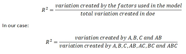
We can also quantitatively assess the quality of the model using the coefficient of determination R2 This coefficient indicates how much of the variation created in that doe was due to the effects included in the model.
A high R2 means that the effects found to be significant explain most of the variation, a low R2 means that there is a lot of unexplained variation (high level of noise).
How to calculate R2?
In Experiment 23=8, variation was potentially created by three main effects: A, B, and C, and four interaction effects: AB, AC, BC, and ABC. To understand their impact on y: powder humidity, we can do two things:
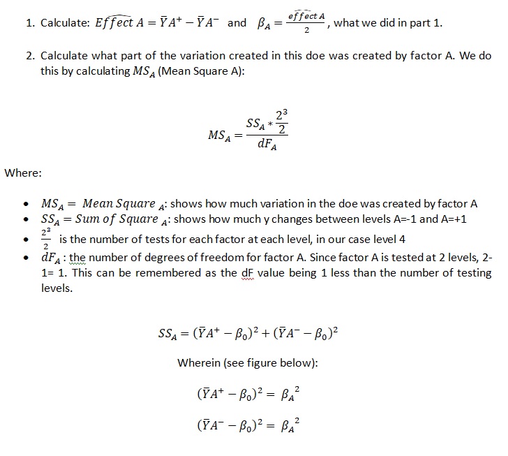
Calculate the effect sizes, i.e., how changing a given effect from -1 to +1 affects the mean y (as shown in Part 1).
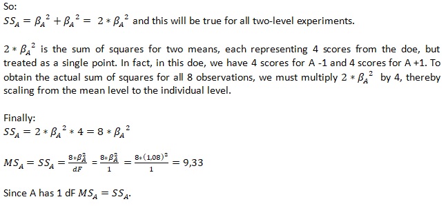
Estimate how much of the variation in the doe was created by each effect.
For example, consider main effect A. To understand the impact of A on y, we can:
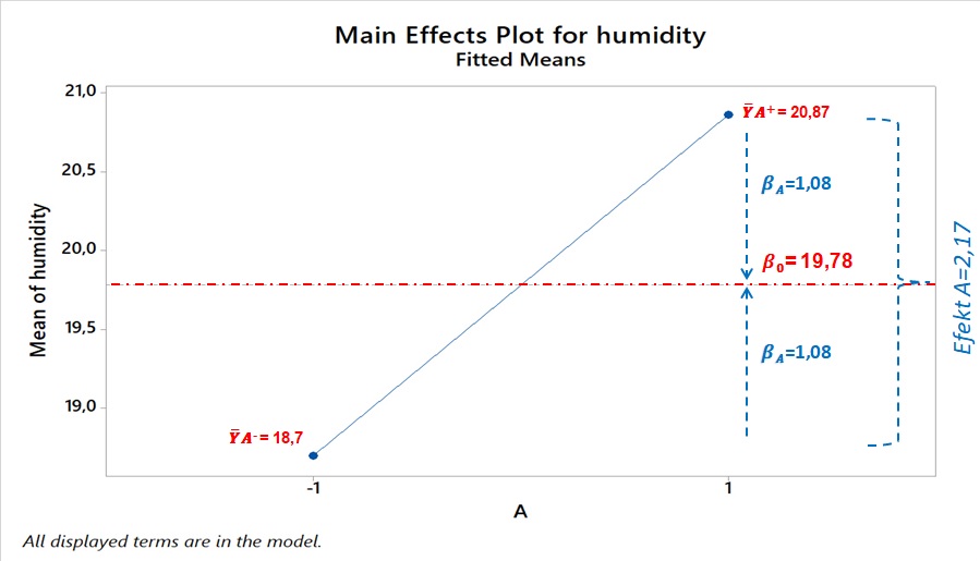
Click to enlarge
The calculation results for all effects including doe are shown in the table below:
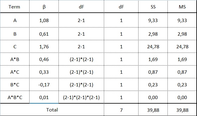
Click to enlarge
We built our prediction equation using A, B and C and the AB interaction, considering the remaining effects, i.e. the remaining interactions, as not significant (not creating variation in this DOE).
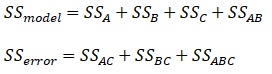
Making calculations using the results in the table above:
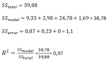
In our example, R2 is 97%. This means that using factors A, B, C, and the AB interaction, we can explain 97% of the variation created in this doe.
The higher the R2, the better? What can we do to improve our unsatisfactory R2? We can add non-significant effects to the model, inflating R2. If we included all seven effects, R2 would be 100%.
But why shouldn’t we do this? Because it makes no sense! If we consider a factor to be non-significant, if it didn’t create variation, it will only clutter the model. Its effect in this doe is considered as noise. If it’s a factor we believe has a significant effect on y, we should test it in the next doe at modified testing levels. However, its presence in the current equation is invalid because it didn’t create variation.
To check whether our equation has been contaminated by non-significant effects, we use the adjusted R2 coefficient of determination. It takes into account not only the SS for individual components of variation, but also corrects for the number of degrees of freedom.
How to calculate R2 – adjusted?
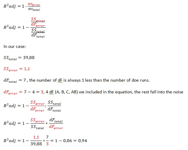
In summary, when a model contains A, B, C, and AB:
R2 = 97%, R2adj = 94%
When the difference between R2 and R2adj is large, it means that the model finds a non-significant effect. In our case, this difference is small, which means that the model is not cluttered.
How does throwing a non-significant effect into the equation affect R2 and R2 adjusted?
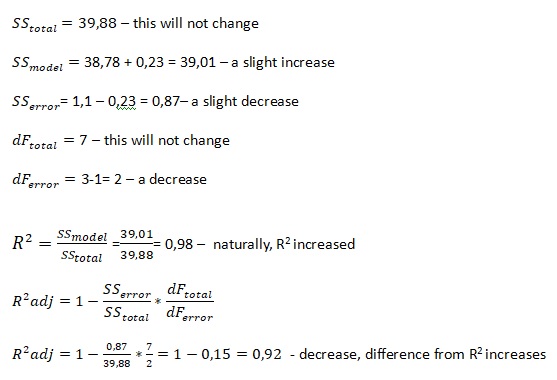
The easiest way to check this is to add a non-significant factor to our equation. Let’s break the model by adding the B*C interaction, for which SSBC = 0.23 (table above).
Comparison
Model containing: A, B, C, AB :R2=97%, R2adj =94%
Model containing: A, B, C, AB, BC :R2=98%, R2adj =92%
Adding BC slightly increased R2. This small difference is due to the very small effect of BC.
R2adj decreased because, despite the small decrease in SSerror, we lost 1 dF in the denominator (3 out of 2). The gain in fit was too small relative to the loss of this dF. Thus, R2adj penalizes insignificant effects in the model.
Questions:
- Does the equation always work?
- What determines whether it works?
